Pre Processing

                                           Pre - Processing

The pre-processing phase in machine learning (ML) is a crucial step where raw data is cleaned and transformed to make it suitable for a machine learning model. This phase involves a series of systematic steps designed to improve the quality and efficiency of the data before it's used for training. Here are the key activities typically involved in the pre-processing phase:

Data Loading / Importing:

Data loading in the context of machine learning involves importing data from various sources into an environment suitable for analysis, typically using libraries and tools like Pandas or TensorFlow. This step includes reading data from different file formats or data streams into structured formats like data frames or tensors. The loaded data is then preprocessed (cleaned, transformed, and sometimes augmented) to make it suitable for training machine learning models. This process is crucial for preparing the data for effective model training, evaluation and deployment، ensuring that it is in an accessible and analyzable state for the algorithms to perform optimally.

When creating machine learning models, you can import data from a variety of file types, each serving different needs and containing different types of data such as CSV, JSON, TXT, IMAGES, SQL, XLS/XLSX.

Understand the Data:

After upload the data you should know the natural of this data, how many columns/rows have, what the datatype for each column and how the data structured.

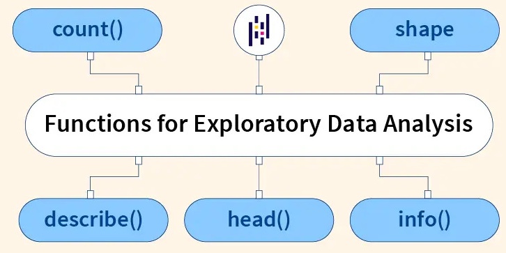
There are a few function & methods in pandas library give you all you want of the data:

• Data.head() : This method show you the first 5 samples of your data, and you can put the number of samples you want in parentheses (), On the other hand you can show the last 5 samples of your data using Data.tail().
• Data.info() : This method show you each column’s datatype, how many samples each column has, how many non-null values and the memory usage of your data, and you can put the verbose, count of column, usage memory and null counts in parentheses ().
• Data.describe() : This method show you general information about your int & float data as maximum value the data have and 'minimum value', 'mean', 'mode', 'std', 'count' and the some percentage of you data 25% , 50%, 75%, and you can put include, exclude and the percentiles in parentheses ().
• Data.count() : This function in Python particularly used with pandas DataFrames, returns the count of non-NA/null observations across the given axis. This means it will show you how many entries are present in each column of your DataFrame that are not empty or null. In parentheses () You can specify the axis along which to count non-null values. By default, axis=0 for counting down the rows for each column. If you set axis=1, it counts across the columns for each row
• Data.shape : This method provides information about the number of rows and columns in a dataFrame quickly and easily, in other concept it's return a tuple representing the dimensionality of the DataFrame.

Missing values:

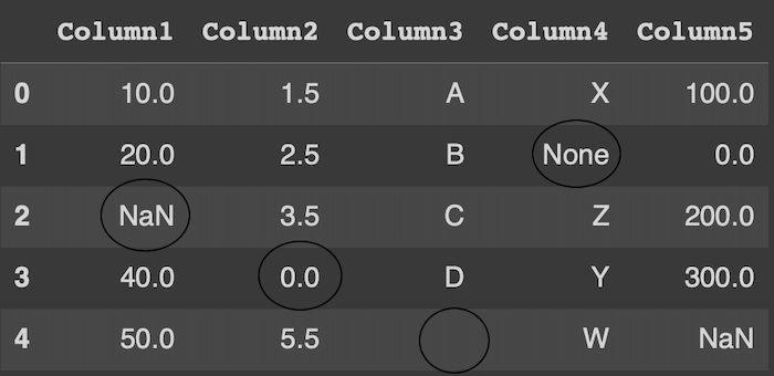
In the world of data science and analytics, encountering missing data is more a rule than an exception. Missing values can skew analysis, lead to incorrect conclusions and generally disrupt the flow of data processing. Addressing these gaps is crucial for maintaining the integrity of your analysis. There are 4 types of these values:

• NaN : NaN stands for "Not a Number" in mathematics. It is a value that is used to represent undefined or unrepresentable results, such as the result of dividing zero by zero or the result of subtracting infinity from infinity. In computing، NaN is often used to indicate an error or undefined result in calculations involving floating-point numbers. When you encounter NaN in calculations, it generally means that the result is not meaningful or cannot be represented as a real number.
• None / Null : Represents an empty value and carry no meaningful information. In Python, None is a special constant that represents the absence of a value. It is often used to signify 'null' or 'nothing' and can be compared to null in other programming languages like Java or JavaScript.
• Empty : An empty string ('' ") in pandas is considered a valid string value and not a null or NaN value. If you need to treat empty strings as missing values, you often need to explicitly convert them to NaN for more consistent data processing and analysis.
• Zero : In most contexts, a zero value (0) is not considered a missing value. It is an actual numeric value that indicates a quantity of zero. However, whether zero should be treated as missing or significant depends on the specific scenario and the nature of the data. For example, in a dataset of adult ages, a zero age is impossible and might actually represent missing or unrecorded data, and it's should converted to NaN to indicate missing data.

If the data has missing values so there are two ways to handle it:

1. Deletion: 

This is a viable strategy for handling null values in a dataset, especially when the dataset is large and the proportion of null values is small. The idea is that removing a small number of records (rows) or features (columns) with missing values will not significantly impact the overall dataset's integrity or the quality of analysis.

1. Row Deletion: Often preferable, as it involves removing specific entries with missing values. This approach is less likely to result in a significant loss of information, especially when the null values are scattered across different rows.
2. Column Deletion: More drastic, this method should be considered when a significant portion of a column's data is missing (e.g., 70-80%). It's more likely to be used when the column is not crucial for the analysis or when its high proportion of missing values would undermine the reliability of any imputation.

Threshold for Deletion: The 5% guideline is a general rule of thumb and not a strict rule. The decision to delete rows or columns based on the proportion of missing values should also consider the dataset's size, the importance of retaining as much data as possible for analysis, and the specific context or domain of the data.

In conclusion if the all null values is present 5% or less you can delete it, For instance, in a dataset with 500 rows, if 25 or fewer rows 5% contain null values, deletion might be a viable option. But If the percentage of null values in the dataset exceeds 5%, deletion might lead to a significant loss of data, which can impact the quality and reliability of any subsequent analysis. In such cases, imputation becomes a more appropriate strategy.

2. Imputation :

This involves replacing missing values with substituted values, such as the mean, median, or mode of the column, or using more sophisticated techniques like regression or machine learning-based imputation. The choice of imputation method depends on the nature of the data and the specific requirements of the analysis. There are a 3 ways to impute the null values depends the column type where the null located.

1. Mode : Get the most occur value.
2. Mean : Calculate the average of the values.
3. Median : The middle value in an ordered set (sorted).

Suppose you have column has these values

[4, 6, 5, 13, 5, 9, 2, 15, 6, 5, 11]

Depends of these values the statics be :

• mode = 5
• mean = 4 + 6 + 5 + 13 + 5 + 9 + 2 + 15 + 6 + 5 + 11 / 11 = 81 / 11 = 7.36
• median = 6

If the null value located in categorical column so you should impute null value via mode statistical measure method which identifies the most frequently occuring value in a column. Like if the column where the null value located contain [Ai “6 times” , Data “8 times” , Cyber “4 times”] the mode in this case impute all the null values here with most common category or class and which is “Data” because its most occurring in the column. But what if your column has [3.786 , 17.23 , 20.21 , 8.9 ] here you have numerical values not categorical so in this case we use either mean or median.

Suppose your null values located in numerical column and you hesitate which one is optimal Mean or Median? you should check the Symmetrically of the data before.

Symmetrically :

Each data has distribution which indicates how the values in that column are spread out or arranged, its a way of describing the characteristics and patterns of data for a specific variable represented by the column.

There two main types of distribution:

1. Normal Distribution:

Normal Distribution which mean the data is symmetrically distributed around the "Mean" such as heights of adult's mean so suppose you have column has heights of random adult mean you’ll find most men will have a height around the average height “175” with fewer men being much shorter or much taller. This distribution often called (Gausian or Bell Curve).

2. Skewed Distribution:

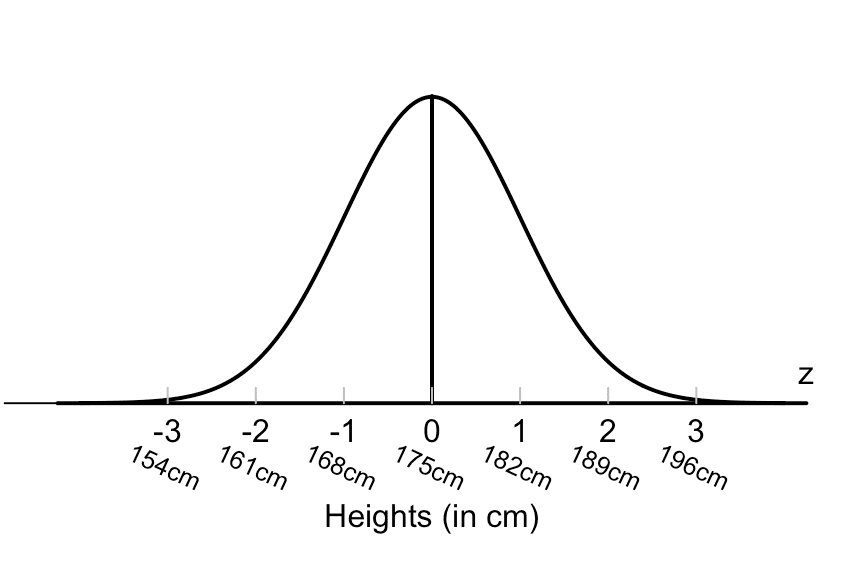
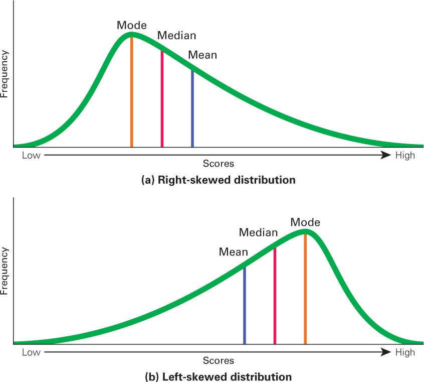
The second type is when the distribution doesn’t symmetrically around the mean so if you have column about age of retirement, its mean you’ll find most people retire at a later age (say, 65 or older), but some retire much earlier due to various factors like health, wealth and personal choice, in this case the distribution of this data be non-symmetric around the mean, it will be right or left symmetric and this type of the distribution called (Skewed) neither left or right Skewed depend on our data.

I hope that now you understand what the distribution and its types mean, so the conclusion about determining when use median or mean.

• if the column distribution is symmetric so you can use mean or median (mean is prefer).
• if the column distribution is left - skewed or right - skewed you should use median.

To solve the skewed problem you should use transformation methods such as logarithmic, square root, or reciprocal transformations for Right-skewed (positively skewed / long tail on the right) These transformations compress large values more than small ones, reducing right skewness.

On another side if your data is skewed for the left (negatively skewed / long tail on the left) you can use square, cube, or exponential transformations. These amplify larger values more than smaller ones, balancing left skewness.

Suppose you have null values and your data is right-skewed, in this case you can do one of two methods:

1. Solve the skewed problem then use mean to impute your data.
2. Use median for imputation then after check the outliers solve and handle the skewed.

Note : keep in mind if you decide use mean to impute your null values is better to check the outliers before handle them because if your data suffering from outliers then the mean of your data be different (mean is sensitive to outliers).

Outliers ( The Silent Killer):

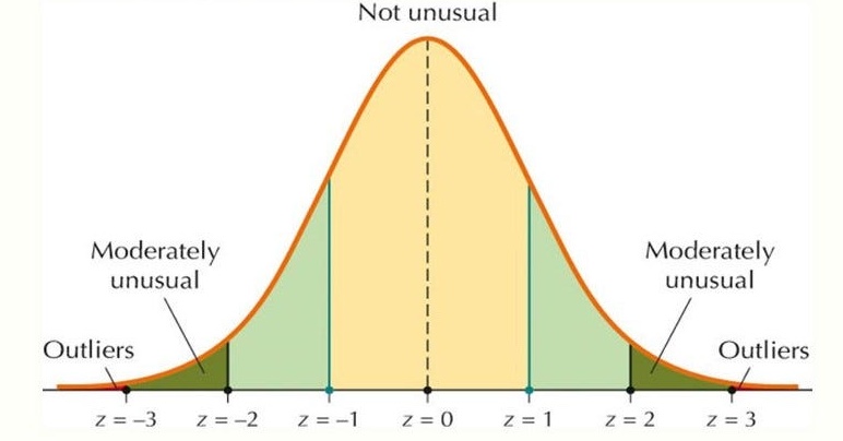
In simple terms, an outlier is an extremely high or extremely low data point relative to the nearest data point and the rest of the neighboring co-existing values in a data graph or dataset you're working with. So the outliers often change the mean of data and due to skewed.

Outliers are extreme values that stand out greatly from the overall pattern of values in a dataset or graph.

Detection:

Detecting outliers in a dataset involves using statistical methods and visualization techniques to identify data points that deviate significantly from the rest of the data. Here are some common methods for outlier detection:

1. Statistical Methods

Statistical Methods is one of methods for outliers detection and we’ll focus on it to determine if our data contain outliers or not, this method can apply through one of these techniques :

A) Z- Score:

• The Z-score represents the number of standard deviations a data point is from the mean.
• Data points with a Z-score greater than 3 or less than -3 are often considered outliers.

B) Interquartile Range (IQR):

• IQR is the range between the first quartile (25th percentile) and the third quartile (75th percentile) of the data.
• Outliers are often defined as data points that fall below Q1 - 1.5IQR or above Q3 + 1.5IQR.

2. Visualization Techniques:

The process of representing data or information in a graphical format, It can involve creating charts, graphs, diagrams, or other visual tools. The visualization of your data can show you the distribution of data points and you can extract the outliers from these visualization. The Visualization Techniques apply through it’s techniques such as:

A) Box Plots:

• Box plots visually show the distribution of the data and its quartiles.
• Data points that appear outside of the whiskers of the box plot can be considered outliers.

B) Scatter Plots:

• Scatter plots can be used to visually inspect the data for outliers, especially in datasets with multiple variables.

3. Machine Learning Methods:

Also we can detect the outliers using ml methods but this method has a lot of drawbacks and this is the common “Complexity and Interpretability”, “Computational Resource and Time” and “Parameter Tuning”.

The methods of machine learning we can use to detect the outliers are:

A) Isolation Forest:

• A tree-based model that isolates outliers by randomly selecting a feature and then randomly selecting a split value between the maximum and minimum values of the selected feature.

B) DBSCAN (Density-Based Spatial Clustering of Applications with Noise):

• A clustering algorithm that separates high-density areas from low-density areas, treating low-density points as outliers.

C) Local Outlier Factor (LOF):

• LOF measures the local density deviation of a given data point with respect to its neighbors. It considers outliers as those points that have a substantially lower density than their neighbors.

Outliers in general can broadly be classified into two categories based on their origin - Genuine outliers and Error outliers, we'll dive further to each one.

1. Genuine Outliers:

Genuine outliers are data points that are unusual but not due to any error or anomaly in data collection or entry. They are legitimate data points that represent extreme cases in the dataset. In a dataset of credit card transactions, a transaction worth $1 million might be a genuine outlier if it represents a legitimate purchase by a very wealthy individual. There is two ways to handle your genuine outliers:

A) Keeping the genuine outliers in your data “when provide valuable information”, let’s say you have dataset on monthly energy consumption by different industries and one industry shows an exceptionally high energy usage for a particular month. This outlier is real and due to this industry starting a new, energy-intensive process that month.

In this case the outliers is kept in the analysis as it provides valuable information about energy demands when industries adopt new processes, because the analysis notes this outlier and its cause, offering insights into how industrial changes impact energy consumption.

B) Transforming the genuine outliers in your data “when it’s have an undue influence on the data” and know what is the origin values for it you can correct them through Logarithmic, square root, or Box-Cox transformations, let’s say you have dataset of finishing times for a large city marathon, and a few runners have significantly longer finishing times than the majority.

These outliers are genuine (not errors) because they represent participants who walked the marathon or faced difficulties, but it doesn’t provide any valuable information. For an analysis focused on competitive running times, these outliers might be excluded since they represent a different category of participants (e.g., walkers or casual participants) and don't inform about the competitive running aspect.

In this case we gonna transform these outliers rather than drop or keep it through Logarithmic, square root, or Box-Cox transformations.

2. Error Outliers:

Error outliers are data points that are unusual due to errors in data collection, processing or entry. They don't reflect the actual distribution of the data. Example of it in a dataset of high school students' ages, an entry of 120 years would be an error outlier, likely due to a data entry mistake. There is two ways to handle your error outliers:

A) Drop (Remove) the outliers are errors or noise (e.g., data entry errors, measurement errors) and when a model is sensitive to outliers.

The common algorithms which sensitive with outliers are :

• Linear Regression
• Logistic Regression
• K-Means Clustering
• Neural Networks

B) Impute the outliers appear to be errors, but you do not want to lose data points. Don’t impute the error outliers with mean because the outliers already changed the mean of your data.

The main problem is what we have to do with outliers, but finding the outliers in our dataset is not a very difficult task. Unfortunately there’s not specific or ways to determine if the outliers is genuine or error neither domain knowledge and your understanding of your data, i know this topic is make confusing and maybe be hard to check the outliers in each time you create a model but don’t afraid 82% prefer to keep the outliers till face a problem or want optimize the model on evaluation stage, so if you don’t have enough time to check the outliers you can keep in whether is genuine or errors and return into it if you face a problem or want optimize your model.

Visualization :

Data visualization is a crucial aspect of machine learning that enables analysts to understand and make sense of data patterns, relationships, and trends. Through data visualization, insights and patterns in data can be easily interpreted and communicated to a wider audience, making it a critical component of machine learning.

Data visualization helps machine learning analysts to better understand and analyze complex data sets by presenting them in an easily understandable format. Data visualization is an essential step in data preparation and analysis as it helps to identify outliers, trends, and patterns in the data that may be missed by other forms of analysis.

With the increasing availability of big data, it has become more important than ever to use data visualization techniques to explore and understand the data. Machine learning algorithms work best when they have high-quality and clean data, and data visualization can help to identify and remove any inconsistencies or anomalies in the data.

This step is not related in specific level on pre-processing phase, it can use in any level of modeling circle to get insights of our work then optimize it, so it's divide into types depends on which step you want to use it :

- Data Understanding

1. Histograms: Used to visualize the distribution of a dataset, showing the frequency of values within a certain range. This is helpful for understanding the skewness and presence of outliers.
2. Line Chart: a line chart (also referred to as a line graph or a trend line) is a type of graphical representation used to visualize the relationship between two variables, typically with one independent variable and one dependent variable.
3. Scatter Plots: Useful for visualizing the relationship between two continuous variables. Scatter plots can help detect any linear or nonlinear relationships, clusters, and outliers.
4. Box Plots: These are used to show the distribution of data in terms of quartiles and to detect outliers effectively.
5. Correlation Heatmaps: Heatmaps can visually represent the correlation matrix of variables, highlighting how variables are related to each other. High correlation coefficients can suggest potential multicollinearity issues.
6. Pair Plots: These show pairwise relationships in a dataset. They can be used to visualize the relationship between each pair of features and the target variable, often as a grid of scatter plots for each pair.

- Model Understanding / Evaluation

1. Confusion Matrix Visualization: A confusion matrix in a graphical format (like a heatmap) helps in understanding the classification performance of a model across different classes.
2. ROC Curve: Receiver Operating Characteristic (ROC) curve is used to visualize the performance of a classifier by plotting the true positive rate against the false positive rate at various threshold settings.
3. Precision-Recall Curve: This is similar to the ROC curve but focuses on the relationship between precision and recall for different threshold levels, useful particularly when classes are imbalanced.
4. Feature Importance Plots: Bar charts or other forms of charts that show the importance or contribution of each feature to the model. This is particularly common with tree-based models like decision trees and random forests.
5. Decision Boundary Visualization: In classification problems, visualizing the decision boundary can help understand how the model divides the feature space and makes predictions.
6. Residual Plots: Useful in regression models to analyze the residuals (errors) of predictions versus actual values to detect patterns that might suggest problems with the model, like non-linearity or heteroscedasticity.

- Model Diagnostics

1. Learning Curves: These plots show the model’s performance on the training set and validation set over time (or over the number of training instances), helping to diagnose issues like overfitting or underfitting.
2. Validation Curves: These are used to visualize the change in training and validation scores with respect to model parameters, useful for hyperparameter tuning.

Duplicates :

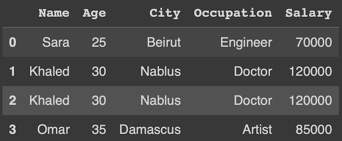
Sometimes due various factors as importing, multiple data sources and systems errors generate duplicate rows which all its values be matches and its implications lead to somethings like skewed analysis so the duplicates can lead to incorrect calculations and analyses, such as inflated sums or averages, misleading statistics, and faulty conclusions. And also lead reduced data quality so the presence of duplicates often signifies broader issues with data management practices, affecting overall data quality. Additionally lead to consume unnecessary storage space and can slow down data processing. So we should remove the duplicates rows in our data if it's found.

Feature Engineering :

After understand the natural of your data, now you should got all insights of what you would to do with the data and determine how can make it more robust and know the low & high important columns. You have three ways to make your data more robust if is applicable :

1. Drop Features :

Suppose you have data which has columns about the salary of each employee in 'X' company, one of these column named “id” of the employee and you know that this column wont effect of my prediction and will be not useful, so you can drop it to make all columns you need it.

2. Add Features :

Assume you have a dataset containing sales data for a company. The dataset includes columns for 'Units Sold' and 'Unit Price'. To evaluate the performance and for further financial analysis, you need to know the total sales amount for each transaction. So you add new column name “Total sales” which contain each unit sold * unit price.

3. Combine Features :

The dataset you have contain three columns "Year", "Month" and "Day", so you can combine all of them into one column to be like this 13/7/2023 instead each number in separate column.

Should i delete the initial columns after combination process / Why ?

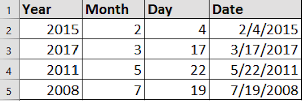
Yes, if you don’t drop the initial columns you’ll face the multicollinearity problem, what is the multicollinearity problem ?

Multicollinearity :

Multicollinearity is a statistical concept commonly encountered in regression analysis. It occurs when two or more predictor variables (independent variables / input / features) in a regression model are highly correlated with each other, meaning that one variable can be linearly predicted from the others with a substantial degree of accuracy. In normal situation the features should doesn’t have any relation between it and another independent column like if you have data about houses price and the columns are num_bathrooms and num_bedrooms and the target is house price, so if when number the bathrooms increase the number of bedrooms increase with it you’re facing the multicollinearity issue, here each column impact with the other column which is has relation with it and with the dependent variable, the relation should be just between independent and dependent variables, and this is called correlation (the primary concept in linear regression).

It is detected using methods like Variance Inflation Factor (VIF) and can be resolved by removing correlated predictors, using principal component analysis, or applying regularization methods. So if the VIF be higher than 5 this indicated the column has correlated with other independent column.

Correlation :

Correlation is a statistical measure that describes the extent to which two variables change together. It ranges from -1 to 1, where 1 indicates a perfect positive linear relationship, -1 indicates a perfect negative linear relationship, and 0 indicates no linear relationship.

The regression tasks on linearity data depends the correlation between individual feature and its target, so if the x variable increase or decrease the target increase or decrease, if the columns doesn’t have correlation with the target variable so it’s not linearity and you shouldn’t use regression - linearity algorithms. The correlation is not the primary key to determine is X column is important or lead to better performance or accuracy, its just determine the linearity relation between the specific column and target, so maybe you have column has strong linearity correlation with target but is irrelevant (called spurious colleration)

Relevant / Irrelevant Features :

Imagine that you have a dataset with various features, including the number of ice cream sales at the beach to predict the number of shark attacks at beaches, when you calculated the correlation between ice cream sales column and shark attacks at beaches column (Target) the result show there are a strong linearity relation between them, lets say when ice cream sales increase do shark attacks. The key factor here is the weather, particularly the temperature. Warm weather leads to more people going to the beach, which in turn leads to an increase in ice cream sales and also increases the likelihood of people swimming in the ocean, where they are at risk of shark attacks.

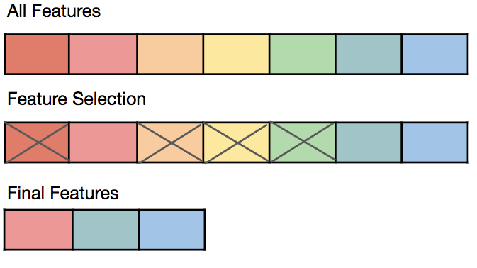
The correlation between ice cream sales and shark attacks is spurious because both are influenced by a third variable (Temperature) not necessarily be in data and there is no direct causal relationship between them, so we should reduce the dimensionality and delete the irrelevant features and keep just the most relevant features for your model which can reduce overfitting and improve model performance, this process is called Feature Selection.

Categorical Features Handling :

Most of machine learning algorithms take just specific datatypes because its depends on mathematical equations, these types are “int” and “float” so if i have any other dtype so i should converting it to numerical format for most algorithms to process it effectively. There are a lot of ways to convert the datatype of specific categorical column to numerical, but these are the most common:

1. One - Hot encoding :

One - Hot encoder is a technique can implemented using libraries such as Scikit-learn in Python to transforms each categorical class into a new binary column, its generally suitable for non-ordinal data such as is your column be about countries names like (Finland, Switzerland, Palestine, Italy) and the ordering here is not important so if i switch between Italy and Finland is anything change ? Of course no, so in this case we’re going to use One - Hot encoder technique.

The mechanism of One - Hot encoder is in each level in the categorical variable, One-Hot Encoding creates a new binary column. This column contains “1” if the original data was of that category, and “0” otherwise.

So in our example the One-Hot Encoding will create four new columns, one for each category, it will have “1” in the 'Palestine' column and “0” in all the “Finland”, “Switzerland'”and “Italy” columns. But what if your data is ordering such as clothes sizes (Small, Medium, Large, XL) here you can’t switch the XL with Small because in this case you re-ordering the normal sizes, in this case the One - Hot encoding doesn’t be good choice and you should use another technique.

NOTE : You should remove/drop the initial country column after encode it to avoid the multicollinearity between the features.

2. Label Encoder :

Is a technique used to convert categorical data into numerical form so that it can be processed by machine learning algorithms that require numerical input. This method involves assigning a unique integer to each category within a column. The integers are usually assigned in an ordinal manner where the first unique category encountered gets encoded as 0, the next as 1, and so forth. This process effectively transforms string labels into a series of numbers, making the data more suitable for algorithms that handle numerical values. Suppose your data about the size of clothes 

The mechanism of Label Encoder is replace the categorical to numeric values so the new column be like this (0, 1, 2, 3) instead (Small, Medium, Large, XL). But what if your data is ordering such as clothes sizes (Small, Medium, Large, XL) here you can’t switch the XL with Small because in this case you re-ordering the normal sizes, in this case the label encoder doesn’t be good choice and you should use another technique.

So the sizes to numeric values, the new column be like this (0, 1, 2, 3) instead (Small, Medium, Large, XL). But what if the data just has two values like Yes/No, Short/Tall or Bad/Good, here in this case the best method is Boolean Encoding because its a simple yet effective way to represent binary categorical data, and its primary advantages are its straightforward interpretability and efficiency in both storage and computation.

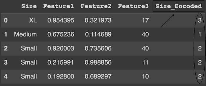
NOTE : You should remove/drop the initial sizes column after encode it to avoid the multicollinearity between the features.

3. Boolean Encoding :

Boolean Encoding is a technique of representing binary categorical data using Boolean values, typically Bad and Good. In the context of data processing and analysis, especially in programming and database management, Boolean Encoding is used to encode categorical variables that have only two categories.

It's specifically used for variables that have only two categories or states. Common examples include Yes/No, True/False, On/Off, or 1/0 scenarios.

The mechanism of this technique is firstly identify the variable in your dataset that has only two distinct categories. Examples include a "Subscribed" column with values "Good" and "Bad", or an "Active" column with values "On" and "Off", then determine the mapping which mean decide how you will map these two categories to Boolean values. Typically, a positive or affirmative category (like "Good", "Active", or "On") is mapped to True, and the negative or inactive category (like "No", "Inactive", or "Off") is mapped to False. Finally convert the categories so apply this mapping to the entire dataset. Every instance of the first category (e.g., "Good") is replaced with True, and every instance of the second category (e.g., "Bad") is replaced with False. After all that the data will be boolean values (True or False) instead (Bad or Good).

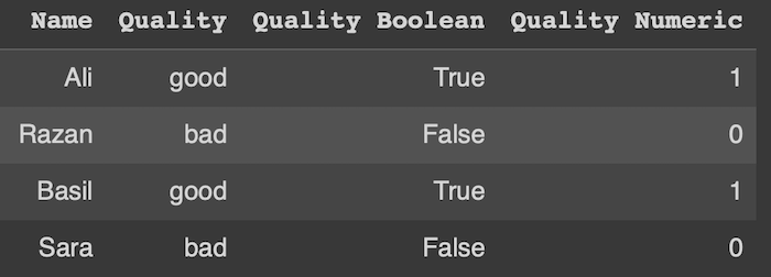
NOTE (1): You should remove/drop the initial quality column after encode it to avoid the multicollinearity between the features.

NOTE (2): IF YOUR DATA IS NON-ORDINAL YOU CAN USE LABEL ENCODING, BUT ON THE ORDINAL DATA YOU SHOULD JUST USE LABEL ENCODING.

After you did all pre-processing techniques now your data is almost ready to use it into the model, so you just at the moment prepare the data itself to entry it into the model, you just want tell the model which columns you want it to be as features and which one want to be target so this step called “Dividing the data”

Dividing the data:

Suppose you have tabular data contain 20 columns and after all pre-processing steps you did surely you know the structure of your data, so lets say you want the column number 7 to be the target column (its not nessecrly the target column always be the last one) and the other columns be the features of your data. Here you tell the model train the features to predict the target and you also shouldn’t tell the model to take all the entire data, in this example you’ll not test your model so after the divide your data to features and target you should tell the model the percentage of the data to take for training and the rest of it keep it for test stage .

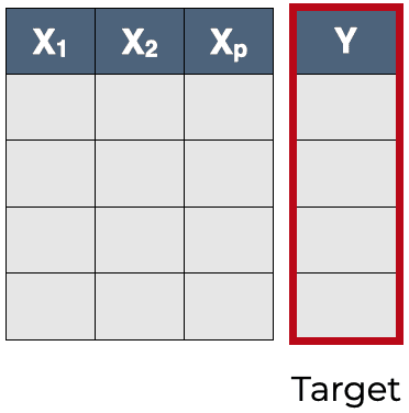
Data Splitting :

For the testing stage you should tell the model how much the data take for training stage and for testing stage, there are three common percentage to split your data :

1. 80% Training, 20% Testing : This is the most common one, a lot of programmer prefer to use it and they see that the training data should be the large as possible to make the model understand the pattern carefully.

2. 70% Training, 30% Testing : Personality always follow this way to give me space if i have issues in evaluation stage to change the ratio as i want, like in the overfitting problem i can increase it to be like the first way, and provides a better balance.

3. 50% Training, 50% Testing : Rarely to use in coding is always used in research paper to focus on the theory not the performance.

Now your data is ready to enter to the model to start the training stage, but wait to reduce the percentage to recheck and evaluate your model if the result is poor i suggest do another step if its found in your data.

Feature Scaling :

Suppose after doing all things your data’s columns be like this, one column’s value range between 2 - 20 and another one column’s values range between 500-5000, in this case your model may face confusing when see the different ranges for each columns to solve this issue you should do feature scaling .

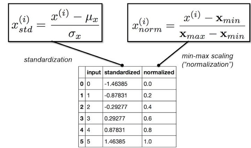
Feature scaling is a method to normalize the range of independent variables or features of data. The primary goal of feature scaling is to ensure that no single feature dominates the others in terms of scale, which can happen when the features have different units or ranges. There are two common types of feature scaling:

1. Normalization :

This technique scales the features to a fixed range, typically 0 to 1. Where the Max(x) and Min(x) are the minimum and maximum values in the feature, respectively. This scaling compresses all the features into the range [0, 1] and is useful when you know the range of the data. Normalization is sensitive to outliers since it directly scales based on the minimum and maximum values of the data.

2. Standardization :

This technique involves rescaling the features so that they have the properties of a standard normal distribution with a mean of 0 and a standard deviation of 1, Standardization is less affected by outliers and is often used when the data does not have a specific range.

There are a lot factors to decide which one the optimal for your case, some people prefer use both of them and compare their performance or combine both and its depend on the nature of each feature, so the choice refer to you. The main factors are :

- Algorithm :

Normalization is better when you use neural network algorithms because algorithms such as neural networks often expect input values in the range of 0 to 1. Normalization is a natural choice in these cases. 

In other hand many machine learning algorithms in libraries like Scikit-learn assume that the input data is standardized. For instance, algorithms like logistic regression, linear regression, and support vector machines perform better with standardized data.

- Outliers :

If you have outliers in your data so the standardization is better than normalization, its mean if your data distribution is Gaussian (normal). In other hand if your data doesn’t have outliers so prefer to use normalization. 

However, the best choice can depend on the specific characteristics of the data and the requirements of the machine learning model being used.

let's emphasize the importance of following these steps in order in pre-processing stage:

1. Data Loading / Importing
2. Understand the Data
3. Duplicate checking
4. Missing values handling
5. Features Engineering
6. Symmetrically / Skewes checking
7. Outliers Detection
8. Linearity checking
9. The Sufficient of Correlation / P > Value 
10. Categorical features converting
11. Multicollinearity checking
12. Divide the data into features “X” and target “Y”
13. Data splitting Training / Testing
14. Features scaling